CONT+CyA+FCCP.csv
CONT+FCCP.csv
H2O2_24hr+FCCP.csv
H2O2_72hr+CyA+FCCP.csv
H2O2_72hr+FCCP.csv

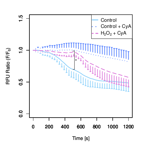
論文作成時のRでのグラフ描画例。gplotsのplotCIとmatrixStatsの関数を使った例。
	  # install.packages("gplots", dependencies = TRUE)
	  # install.packages("matrixStats", dependencies = TRUE)
	  library(gplots)
	  library(matrixStats)

	  cls <- function(){ while(dev.cur() > 1) {dev.off()} }
	  cls()

	  par_set <- function(){
	  par(pin=c(4.3, 4.3))
	  par(mai=c(1,1,0.5,0.5)) $ BLUR
	  par(ps=13)
	  }

	  c1 <- read.table("CONT+FCCP.csv",sep=",")
	  c2 <- read.table("H2O2_24hr+FCCP.csv",sep=",")
	  c3 <- read.table("H2O2_72hr+FCCP.csv",sep=",")
	  c1a<- read.table("CONT+CyA+FCCP.csv",sep=",")
	  c3a<- read.table("H2O2_72hr+CyA+FCCP.csv",sep=",")

	  par_set()
	  matplot(c1[2:42,1],c1[2:42,2:79],xlim=c(0,1200),ylim=c(0.0,1.5),type="l",col=1,lwd=1,lty=1,ylab=expression(paste(paste("RFU Ratio (F/",F[0]),")")),xlab="Time [s]")
	  dev.copy2eps(device=postscript, file="CONT+FCCP.eps", width=5, height=5, family="Helvetica")
	  cls()

	  par_set()
	  matplot(c1[2:42,1],c1[2:42,2:79],xlim=c(0,1200),ylim=c(0.0,1.5),type="l",col=rainbow(8),lwd=1,lty=1,ylab=expression(paste(paste("RFU Ratio (F/",F[0]),")")),xlab="Time [s]")
	  dev.copy2eps(device=postscript, file="CONT+FCCP_color.eps", width=5, height=5, family="Helvetica")
	  cls()
下付き文字はexpression()使うと良い。
	  par_set()
	  par(ps=12)
	  matplot(c1[2:42,1],rowMeans(c1[2:42,2:79]),xlim=c(0,1200),ylim=c(0.0,1.5),type="l",col="lightskyblue",lwd=2,lty=1,xlab="",ylab="")
	  par(new=T)
	  plotCI(as.numeric(data.matrix(c1[2:42,1])),rowMeans(c1[2:42,2:79]),xlim=c(0,1200),ylim=c(0.0,1.5),type=NA,lwd=2,col="lightskyblue",liw=rowSds(data.matrix(c1[2:42,2:79])),uiw=NULL,xlab="",ylab="",sfrac=0.003)
	  par(new=T)

	  matplot(c1a[2:42,1],rowMeans(c1a[2:42,2:50]),xlim=c(0,1200),ylim=c(0.0,1.5),type="l",col="royalblue1",lwd=2,lty=3,ylab=expression(paste(paste("RFU Ratio (F/",F[0]),")")),xlab="Time [s]")
	  par(new=T)
	  plotCI(as.numeric(data.matrix(c1a[2:42,1])),rowMeans(c1a[2:42,2:50]),xlim=c(0,1200),ylim=c(0.0,1.5),type=NA,lwd=2,col="royalblue1",uiw=rowSds(data.matrix(c1a[2:42,2:50])),liw=NULL,xlab="",ylab="",sfrac=0.003)
	  par(new=T)

	  matplot(c3a[2:42,1],rowMeans(c3a[2:42,2:60]),xlim=c(0,1200),ylim=c(0.0,1.5),type="l",col="orchid",lwd=2,lty=5,ylab=expression(paste(paste("RFU Ratio (F/",F[0]),")")),xlab="Time [s]")
	  par(new=T)
	  plotCI(as.numeric(data.matrix(c3a[2:42,1])),rowMeans(c3a[2:42,2:60]),xlim=c(0,1200),ylim=c(0.0,1.5),type=NA,lwd=2,col="orchid",liw=rowSds(data.matrix(c3a[2:42,2:60])),uiw=NULL,xlab="",ylab="",sfrac=0.003)

	  legend("topright", legend = c("Control", "Control + CyA", expression(paste("", paste(paste(H[2],O[2])," + CyA"))) ),
	  pch = "", lwd= c(3,3,3), lty = c(1,3,6), bg="white", y.intersp=1.8, text.width=strwidth("Control + CyA")*1.6, col=c("lightskyblue","royalblue1","orchid"))

	  segments(500,0.7,  520,0.7)
	  segments(500,0.99, 520,0.99)
	  segments(520,0.99, 520,0.7)

	  text(525,0.82, "*", pos=4, cex=1, offset=0)

	  dev.copy2eps(device=postscript, file="CONT_H2O2_CyA_color_rev.eps", width=5, height=5, family="Helvetica")
	  cls()
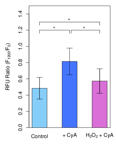
一般的にはarrows()を使う。有意差を示す棒は調整しないといけないことが多い。今回は自前でdrawbraced()を作って対処した。
	  par_set()
	  par(pin=c(3.3, 4.3))
	  par(mai=c(1,1,0.5,0.5)) $ BLUR
	  par(mar=c(3,5,1,1)) $ BLUR

	  c1n_v <- unlist(c1[42:42,2:79],use.names=F)
	  c1a_v <- unlist(c1a[42:42,2:50],use.names=F)
	  c2n_v <- unlist(c2[42:42,2:46],use.names=F)
	  c3n_v <- unlist(c3[42:42,2:64],use.names=F)
	  c3a_v <- unlist(c3a[42:42,2:60],use.names=F)
	  t.test(c1n_v, c3a_v,var.equal=F)
	  t.test(c1a_v, c3a_v,var.equal=F)
	  t.test(c1n_v, c1a_v,var.equal=F)

	  mean_v <- c(mean(c1n_v),mean(c1a_v),mean(c3a_v))
	  stde_v <- c(sd(c1n_v),sd(c1a_v),sd(c3a_v))

	  B <- barplot(mean_v, ylim=c(0.0,1.5), ,ylab=expression( paste(paste(paste(paste("RFU Ratio (", F[1200]),"/"),F[0]),")") ), space=1, col=c("lightskyblue","royalblue1","orchid"),
	  names.arg=c("Control","+ CyA", expression(paste(paste(H[2],O[2])," + CyA"))), xpd=F)
	  arrows(B, mean_v - stde_v, B, mean_v + stde_v, angle = 90, length = 0.1)
	  arrows(B, mean_v + stde_v, B, mean_v - stde_v, angle = 90, length = 0.1)
	  box("plot",lty=1)

	  drawbraced <- function(x1,x2,y) {
	  segments(x1,y, x2,y)
	  segments(x1,y, x1,y-0.04)
	  segments(x2,y, x2,y-0.04)
	  }

	  drawbraced(1.5,3.5,1.2)
	  text(2.4,1.21, "*", pos=4, cex=1, offset=0)

	  drawbraced(3.6,5.5,1.2)
	  text(4.4,1.21, "*", pos=4, cex=1, offset=0)

	  drawbraced(1.5,5.5,1.3)
	  text(3.4,1.31, "*", pos=4, cex=1, offset=0)

	  dev.copy2eps(device=postscript, file="CONT+H2O2_BARPLOT_color.eps", width=4, height=5, family="Helvetica")
	  cls()
On Sunday 01 April 2007, chromatic wrote:
> On Saturday 31 March 2007 15:26, Yuval Kogman wrote:
> > uses_version_control sounds more like lacks_manifest_skip_file which
> > should deduct kwalitee IMHO.
>
> Maybe so, but how else can CPANTS detect that you use the world's most
> advanced version control system: CVS?
>

Are you kidding?

CVS is not advanced as:

1. Microsoft Visual SourceSafe - the only sane choice for good data integrity
and portability.

2. tarballs/zip-files and patches. This one excels in convenience, and
robustness.

CVS is a very advanced version control system, however. I do wish that
Subversion (which is a VCS that I have to use against my will) was as good as
it is.

    -- Shlomi Fish answering to chromatic on 01-April-2007

    -- Shlomi Fish
    -- "Re: New CPANTS metrics" ( http://www.nntp.perl.org/group/perl.qa/2007/03/msg8491.html )